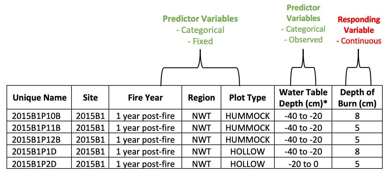
A sample of the data used for objective 1 and 2 are displayed in the following tables which include additional information on our variables.
Objective 1
Table 1. A sample of the dataset sampling units used for objective 1 highlighting site 2011B2-1.
Objective 2
Table 2. A sample of the dataset sampling units used for objective 2 highlighting site 2011B2-1.
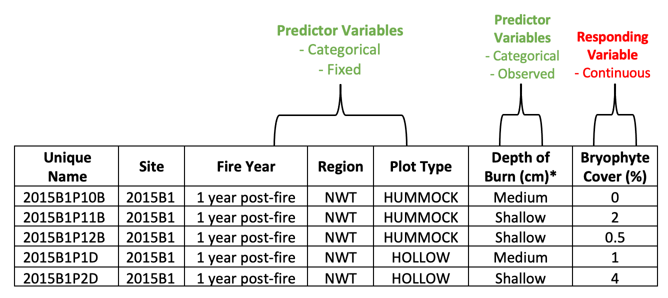
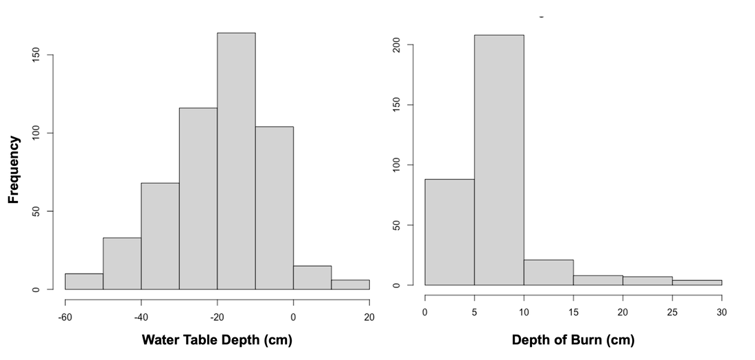
Figure 4. Displays 2 histograms used to categorize continuous variables into categorical variables. The first is water table depth measured in cm, which is grouped into 4 categories; -60 to -40, -40 to -20, -20 to 0, and 0+. The second histogram is of depth of burn measured in cm, which is grouped into 3 categories; Shallow (0-5 cm), Medium (5-10 cm), and Deep (10+ cm).
Frequency of water table levels and depth of burn are displayed in the two histograms in Figure 4. These histograms were used to turn these two continuous variables into discrete variables for the two objectives (water table level for objective 1 and depth of burn for objective 2). Depth of burn is used as a poxy to represent fire severity and was kept as a continuous responding variable for objective 1, then categorized as a discrete variable for objective 2.
Water table depth was categorized into 4 categories: -60 to -40, -40 to -20, -20 to 0, and 0+. The water table depth histogram is slightly skewed to the right but has a fairly normal distribution. The deepest depth of burn was categorized as a depth 10 cm+ and it labelled as Deep. This depth is used as an indication of the most severe fires. 5 to 10 cm depth of burn was labelled as Medium and used as an indication of medium fire severities. Lastly, 0 to 5 cm depth of burn was labelled as shallow and used as an indication of the least severe fires. The depth of burn histogram is skewed to the left and indicates a non-normal distribution for our depth of burn measurements across all the burn sites.
A limitation of our data that could offer a possible explanation for the skewedness of our depth of burn measurements is that our sampling units were observed from natural events that were not controlled. Therefore, the number of sites representing each depth of burn category was limited to recent natural events in similar geographical locations. With that in mind we also do not have the same number of sites for each year post fire which is also a limitation of our dataset.
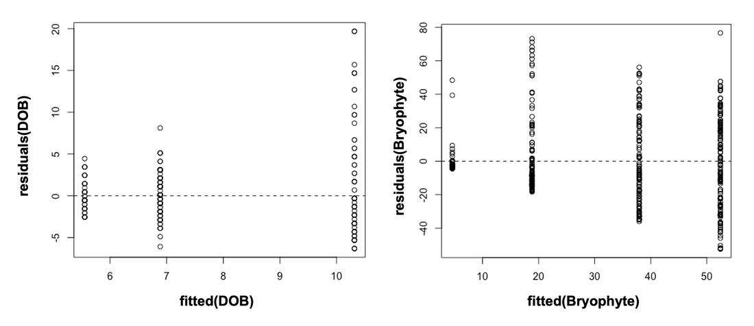
Figure 5. Residual plots showing the normality and homogeneity of variances for our responding variables depth of burn (left) and bryophyte cover (right).
We evaluated our responding variables to see if they met the ANOVA’s assumptions of normality and homogeneity of variances by creating residual plots. As shown in Figure 5, the depth of burn values are not normally distributed as shown by the left skew, and the wedge shape suggests that larger depth of burn values are more variable, violating homogeneity. As for bryophyte cover, the data is primarily normal but has a similar violation of homogeneity (Figure 5). Despite not meeting the ANOVA assumptions, we did not transform the data since it did not significantly change the p-values values or CIs, transformations reduce statistical power, and due to the principles of the central limit theorem.
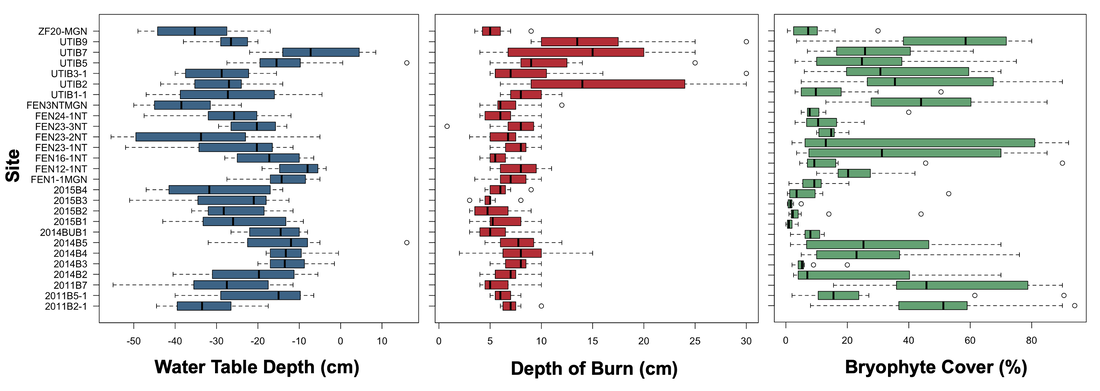 Figure 6. Water table depth (cm), depth of burn (cm) and bryophyte cover (%) value ranges for each individual burn site in our study.
The plot measurements of water table depth, depth of burn and bryophyte cover as continuous variables were averaged for each burn site (Figure 6). The preliminary boxplot analysis is used to look for any visual relationship between low water table depth, deep depth of burns and therefore low bryophyte cover. There appears to be no obvious visualization of such a relationship illustrated in Figure 6. Visualization might be limited due to the large range of values within each site and the number of outliers.
The boxplots displaying depth of burn in Figure 6 illustrates the same non-normal distribution of our data as the depth of burn histogram in Figure 4. Additionally, the water table depth boxplot shows that water table values varied considerably within sites but did not vary much between sites. From the bryophyte cover histogram in Figure 6, we determined that our bryophyte cover data has a non-normal distribution as the spread of error bars is large.
The boxplots displaying depth of burn in Figure 6 illustrates the same non-normal distribution of our data as the depth of burn histogram in Figure 4. Additionally, the water table depth boxplot shows that water table values varied considerably within sites but did not vary much between sites. From the bryophyte cover histogram in Figure 6, we determined that our bryophyte cover data has a non-normal distribution as the spread of error bars is large.
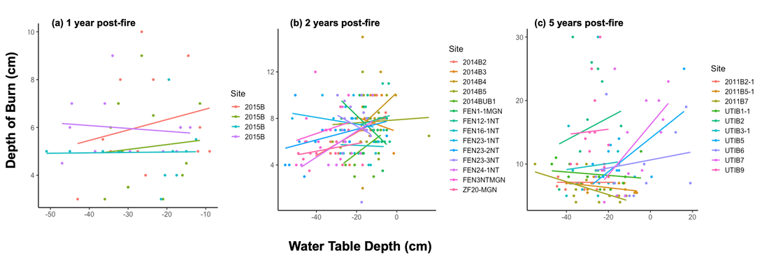
Figure 7. Scatterplots illustrating the relationship between water table depth (cm) and depth of burn (cm) for fire events 1 year post-fire (a), 2 years post-fire (b), and 5 years post-fire (c).
Our second preliminary analysis is displayed in Figure 7 illustrating the relationship of water table depth on depth of burn grouped into the 3 post fire categories. Any consistent visualization of depth of burn increasing as water table depth decreased cannot be seen in these scatterplots (Figure 7). Multiple negative and positive trend lines exist with varying slopes, including some near horizontal trendlines. Many of the sites also have lots of their plot values far from apart and far from the created trendline.
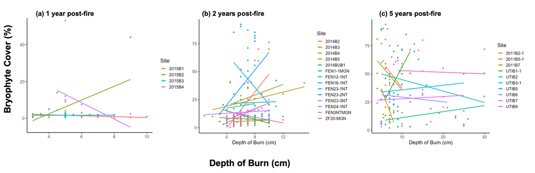
Figure 8. Scatterplots illustrating the relationship between depth of burn (cm) and bryophyte cover (%) for fire events 1 year post-fire (a), 2 years post-fire (b), and 5 years post-fire (c).
Our third preliminary analysis is displayed in Figure 8 illustrating the relationship of depth of burn on percent bryophyte cover grouped into the three post fire categories. Any consistent visualization of bryophyte cover decreasing with deeper depth of burn measurements cannot be seen in these scatterplots (Figure 8). Multiple negative and positive trend lines exist with varying slopes, including some near horizontal trendlines. Many of the sites that were 5 years post-fire have lots of their plot values far from apart and far from the created trendline. Some sites that were 2 years post-fire have plot measurements that are close together while others do not. The four sites from 1 year post-fire events have most of their plot measurements very close to their trend lines, but of those four site there is a positive relationship, a negative relationship and two near horizontal relationships.
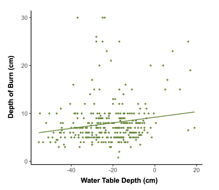
Figure 9. Scatterplot of water table depth (cm) effects on depth of burn (cm) combining all plot values from all sites.
|
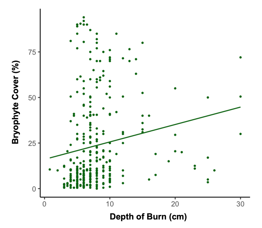
Figure 10. Scatterplot of depth of burn (cm) effects on bryophyte cover (%) combining all plot values from all sites.
|
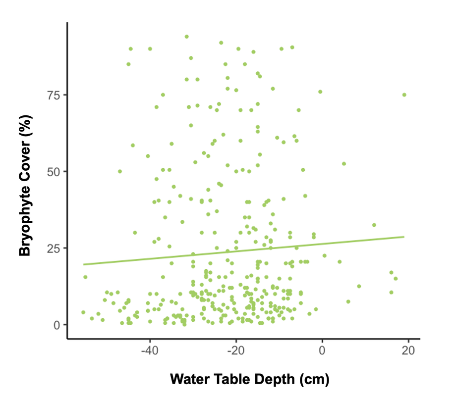
Figure 11. Scatterplot of water table depth (cm) effects on bryophyte cover (%) through the inferred relationship of the two objectives combining all plot values from all sites.
|
Our forth preliminary analysis is a visualization of the relationships we are exploring on a landscape level combining all plot values from all sites (Figures 9, 10, and 11). Scatterplots of the two relationships we are exploring as our two objectives (Figures 9 and 10) plus the implied relationship combining the two objectives (Figure 11) show no obvious visual relationship.
The trendlines are impacted by outliers and the values of individual plots do not show any obvious positive or negative relationship. Figure 9 values mostly display a horizontal trend and Figure 10 values mostly display a vertical trend which gives us no relationship for either. Figure 11 is also so highly scattered that no relationship can be inferred.
The trendlines are impacted by outliers and the values of individual plots do not show any obvious positive or negative relationship. Figure 9 values mostly display a horizontal trend and Figure 10 values mostly display a vertical trend which gives us no relationship for either. Figure 11 is also so highly scattered that no relationship can be inferred.
